Near-Death Experiences
Tidy Tuesday for July 21st, 2026
Near-Death Experiences
Irene Morse
Setup and Introduction
Acknowledgements: I used GPT-5.5-mini to assist with some elements of this post, especially the code for generating plots.
import pandas as pd
import numpy as np
import matplotlib.pyplot as plt
import seaborn as sns
nde_experiences = pd.read_csv('https://raw.githubusercontent.com/rfordatascience/tidytuesday/main/data/2026/2026-07-21/nde_experiences.csv')
nde_experiences.head()
| entry_id | gender | classification | country | category | language | greyson_score | post_date | exp_date | narrative_length | ai_obe | ai_unity | ai_hellish | ai_clinical | ai_esp | ai_past_lives | ai_world_future | ai_aliens | |
|---|---|---|---|---|---|---|---|---|---|---|---|---|---|---|---|---|---|---|
| 0 | 1 | M | NDE | Soviet Union | NDE | english | 0.0 | 1999-02-07T00:00:00Z | NaN | 7146 | True | True | False | True | False | False | False | False |
| 1 | 2 | F | NDE | United States | NDE | english | 3.0 | 1999-02-07T00:00:00Z | 1960-01-18T00:00:00Z | 8188 | True | False | False | True | False | False | False | False |
| 2 | 3 | F | NDE | United States | NDE | english | 17.0 | NaN | 1975-09-17T00:00:00Z | 12889 | True | False | False | True | False | False | False | False |
| 3 | 4 | M | NDE | Vietnam | NDE | english | 0.0 | 1999-02-07T00:00:00Z | 1969-05-03T00:00:00Z | 9449 | True | True | False | True | False | False | False | False |
| 4 | 5 | F | NDE | NaN | NDE | english | 0.0 | 2008-01-13T00:00:00Z | NaN | 3579 | False | False | False | True | False | False | False | False |
For this week’s Tidy Tuesday dataset, I’m interested in exploring the role of country and language as predictors of certain kinds of near-death experiences (NDEs). Do people from certain countries report certain types of NDEs more frequently? And are certain types of NDEs more prevalent in certain languages?
Part 1: Country Analysis
Let’s start by investigating the countries present in the data.
nde_experiences['country'].value_counts()
| count | |
|---|---|
| country | |
| United States | 390 |
| Canada | 28 |
| Australia | 26 |
| France | 24 |
| England | 8 |
| ... | ... |
| Brazil | 1 |
| Kentucky | 1 |
| South Africa | 1 |
| Ukraine | 1 |
| Dominican Republic | 1 |
64 rows × 1 columns
# check for NAs
nde_experiences['country'].isna().sum()
np.int64(8)
Based on the descriptive statistics so far, I will remove countries that have less than 10 entries, two misspelled countries, as well as the 8 NA values.
nde_experiences.shape
(589, 18)
nde_countries_raw = nde_experiences.groupby('country').filter(lambda x: len(x) >= 10)
nde_countries_raw.shape
(468, 18)
mask = ~nde_countries_raw['country'].isin(['U', 'unknown'])
nde_countries_raw = nde_countries_raw[mask]
nde_countries_raw.shape ## it appears that the misspelled countries were already removed when I removed countries by count
(468, 18)
mask = nde_countries_raw['country'].notna()
nde_countries_raw = nde_countries_raw[mask]
nde_countries_raw.shape ## it appears that the NA values were already removed when I removed countries by count
(468, 18)
Next I will reshape the data to prepare for plotting.
nde_countries = nde_countries_raw.groupby('country').agg(
    ai_obe_count=('ai_obe', 'sum'),
    ai_unity_count=('ai_unity', 'sum'),
    ai_hellish_count=('ai_hellish', 'sum'),
    #ai_clinical_count=('ai_clinical', 'sum'),
    ai_esp_count=('ai_esp', 'sum'),
    ai_past_lives_count=('ai_past_lives', 'sum'),
    ai_world_future_count=('ai_world_future', 'sum'),
    ai_aliens_count=('ai_aliens', 'sum')
).reset_index()

nde_countries.head()
| country | ai_obe_count | ai_unity_count | ai_hellish_count | ai_esp_count | ai_past_lives_count | ai_world_future_count | ai_aliens_count | |
|---|---|---|---|---|---|---|---|---|
| 0 | Australia | 16 | 4 | 4 | 6 | 1 | 1 | 0 |
| 1 | Canada | 16 | 3 | 0 | 5 | 0 | 3 | 2 |
| 2 | France | 11 | 7 | 1 | 8 | 0 | 0 | 0 |
| 3 | United States | 232 | 58 | 30 | 59 | 16 | 20 | 2 |
# normalize the data because some countries just have more entries than others
normalization_vector = nde_countries_raw['country'].value_counts().sort_index().to_numpy()
print(normalization_vector)
[ 26 28 24 390]
# normalize the data because some countries just have more entries than others
numeric_cols = nde_countries.select_dtypes(include='number').columns

nde_countries[numeric_cols] = (
    nde_countries[numeric_cols]
    .div(normalization_vector, axis=0)
)

nde_countries.head()
| country | ai_obe_count | ai_unity_count | ai_hellish_count | ai_esp_count | ai_past_lives_count | ai_world_future_count | ai_aliens_count | |
|---|---|---|---|---|---|---|---|---|
| 0 | Australia | 0.615385 | 0.153846 | 0.153846 | 0.230769 | 0.038462 | 0.038462 | 0.000000 |
| 1 | Canada | 0.571429 | 0.107143 | 0.000000 | 0.178571 | 0.000000 | 0.107143 | 0.071429 |
| 2 | France | 0.458333 | 0.291667 | 0.041667 | 0.333333 | 0.000000 | 0.000000 | 0.000000 |
| 3 | United States | 0.594872 | 0.148718 | 0.076923 | 0.151282 | 0.041026 | 0.051282 | 0.005128 |
Now let’s plot!
cols = [
    'ai_obe_count',
    'ai_unity_count',
    'ai_hellish_count',
    #'ai_clinical_count',
    'ai_esp_count',
    'ai_past_lives_count',
    'ai_world_future_count',
    'ai_aliens_count'
]

heatmap_data = nde_countries.set_index('country')[cols]
col_order = heatmap_data.mean().sort_values(ascending=False).index
heatmap_data = heatmap_data[col_order]

# Clean column names for display
heatmap_data.columns = (
    heatmap_data.columns
    .str.replace('ai_', '')
    .str.replace('_count', '')
    #.str.replace('_', ' ')
    #.str.title()
)

plt.figure(figsize=(10, 8))

sns.heatmap(
    heatmap_data,
    annot=True,
    fmt='g',
    cmap='viridis'
)

plt.xlabel('Experience Type')
plt.xticks(rotation=45, ha='right', fontsize=10)
plt.ylabel('Country')
plt.tight_layout()
plt.show()
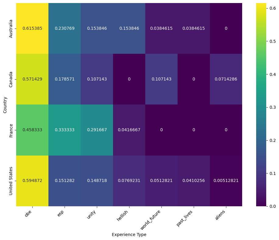
Based on this heatmap, it looks like out-of-body experiences are the most freqently reported feature of NDEs across all countries, followed by extrasensory perception. Interestingly, the NDEs of French people exhibit increased variation in types of experiences when compared to those of Australians, Canadans, and Americans. French NDEs were less skewed toward out-of-body experiences and were more likely to include elements of extrasensory perception and feelings of unity or oneness.
Part 2: Language Analysis
Let’s again start with some descriptive analysis.
nde_experiences['language'].value_counts()
| count | |
|---|---|
| language | |
| english | 549 |
| fr | 18 |
| es | 5 |
| ar | 3 |
| sv | 2 |
| french | 2 |
| español | 2 |
| nl | 2 |
| français | 1 |
| id | 1 |
| portuguese | 1 |
| spanish | 1 |
| german | 1 |
| nederlands | 1 |
nde_experiences['language'].isna().sum()
np.int64(0)
Luckily there are no NA values in the language column! But we still need to clean up the language entries a bit.
# recode certain language values
nde_languages_raw = nde_experiences.copy()
nde_languages_raw['language'] = nde_experiences['language'].replace({
    'fr': 'french',
    'es': 'spanish',
    'ar': 'arabic',
    'sv': 'swedish',
    'español': 'spanish',
    'nl': 'dutch',
    'français': 'french',
    'id': 'indonesian',
    'nederlands': 'dutch'
})
nde_languages_raw['language'].value_counts() ## much better!
| count | |
|---|---|
| language | |
| english | 549 |
| french | 21 |
| spanish | 8 |
| dutch | 3 |
| arabic | 3 |
| swedish | 2 |
| indonesian | 1 |
| portuguese | 1 |
| german | 1 |
nde_languages_raw.shape
(589, 18)
# remove languages that have less than 5 instances
nde_languages_raw = nde_languages_raw.groupby('language').filter(lambda x: len(x) >= 5)
nde_languages_raw.shape ## only 3 languages removed
(578, 18)
Just as with the country analysis, I will reshape the data to facilitate plotting.
nde_languages = nde_languages_raw.groupby('language').agg(
    ai_obe_count=('ai_obe', 'sum'),
    ai_unity_count=('ai_unity', 'sum'),
    ai_hellish_count=('ai_hellish', 'sum'),
    #ai_clinical_count=('ai_clinical', 'sum'),
    ai_esp_count=('ai_esp', 'sum'),
    ai_past_lives_count=('ai_past_lives', 'sum'),
    ai_world_future_count=('ai_world_future', 'sum'),
    ai_aliens_count=('ai_aliens', 'sum')
).reset_index()

nde_languages.head()
| language | ai_obe_count | ai_unity_count | ai_hellish_count | ai_esp_count | ai_past_lives_count | ai_world_future_count | ai_aliens_count | |
|---|---|---|---|---|---|---|---|---|
| 0 | english | 318 | 89 | 42 | 84 | 18 | 26 | 5 |
| 1 | french | 11 | 4 | 1 | 5 | 0 | 1 | 0 |
| 2 | spanish | 3 | 1 | 2 | 0 | 0 | 0 | 0 |
# normalize the data because some languages just have more entries than others
normalization_vector = nde_languages_raw['language'].value_counts().sort_index().to_numpy()
print(normalization_vector)
[549 21 8]
# normalize the data because some languages just have more entries than others
numeric_cols = nde_languages.select_dtypes(include='number').columns

nde_languages[numeric_cols] = (
    nde_languages[numeric_cols]
    .div(normalization_vector, axis=0)
)

nde_languages.head()
| language | ai_obe_count | ai_unity_count | ai_hellish_count | ai_esp_count | ai_past_lives_count | ai_world_future_count | ai_aliens_count | |
|---|---|---|---|---|---|---|---|---|
| 0 | english | 0.579235 | 0.162113 | 0.076503 | 0.153005 | 0.032787 | 0.047359 | 0.009107 |
| 1 | french | 0.523810 | 0.190476 | 0.047619 | 0.238095 | 0.000000 | 0.047619 | 0.000000 |
| 2 | spanish | 0.375000 | 0.125000 | 0.250000 | 0.000000 | 0.000000 | 0.000000 | 0.000000 |
Ready to plot!
cols = [
    'ai_obe_count',
    'ai_unity_count',
    'ai_hellish_count',
    #'ai_clinical_count',
    'ai_esp_count',
    'ai_past_lives_count',
    'ai_world_future_count',
    'ai_aliens_count'
]

heatmap_data = nde_languages.set_index('language')[cols]
col_order = heatmap_data.mean().sort_values(ascending=False).index
heatmap_data = heatmap_data[col_order]

# Clean column names for display
heatmap_data.columns = (
    heatmap_data.columns
    .str.replace('ai_', '')
    .str.replace('_count', '')
    #.str.replace('_', ' ')
    #.str.title()
)

plt.figure(figsize=(10, 8))

sns.heatmap(
    heatmap_data,
    annot=True,
    fmt='g',
    cmap='viridis'
)

plt.xlabel('Experience Type')
plt.xticks(rotation=45, ha='right', fontsize=10)
plt.ylabel('Language')
plt.tight_layout()
plt.show()
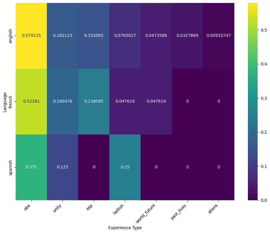
Just like with the country analysis, out-of-body experiences are the most common feature of all NDE narratives. In this langauge analysis, French and Spanish exhibit more variation than English. It is particularly interesting that Spanish narratives are significantly more likely to include distressing or hellish imagery.
Part 3: Over-Time Analysis of “Hellish” NDEs
The analysis thus far has prompted me to consider one new question: How have “hellish” NDEs changed over time? Thanks to Pew’s survey research, we know that the number of Americans identifying as Christian has decreased over time, and Europe has followed similar trends.

Based on these trends, I predict that hellish NDEs will have decreased over time, but let’s check in out!
# extract year from date of NDE
nde_experiences['exp_date'] = pd.to_datetime(nde_experiences['exp_date'])
nde_experiences['year'] = nde_experiences['exp_date'].dt.year
mask = nde_experiences['year'].notna()
nde_experiences_time = nde_experiences[mask]
print(nde_experiences.shape)
print(nde_experiences_time.shape)  ## removed 76 NA values
(589, 19)
(513, 19)
nde_experiences_time = nde_experiences_time.groupby('year').agg(
    ai_hellish_count=('ai_hellish', 'sum')
).reset_index()

nde_experiences_time.describe()
| year | ai_hellish_count | |
|---|---|---|
| count | 67.000000 | 67.000000 |
| mean | 1981.179104 | 0.537313 |
| std | 21.085630 | 1.004963 |
| min | 1936.000000 | 0.000000 |
| 25% | 1964.500000 | 0.000000 |
| 50% | 1981.000000 | 0.000000 |
| 75% | 1997.500000 | 1.000000 |
| max | 2024.000000 | 5.000000 |
plt.figure(figsize=(10, 5))

# base scatterplot
plt.plot(nde_experiences_time['year'], nde_experiences_time['ai_hellish_count'], marker='o')

# Fit quadratic polynomial
coeffs = np.polyfit(nde_experiences_time['year'], nde_experiences_time['ai_hellish_count'], 2)
poly = np.poly1d(coeffs)

# Create smooth x values for plotting the curve
x_fit = np.linspace(nde_experiences_time['year'].min(), nde_experiences_time['year'].max(), 300)
y_fit = poly(x_fit)

# Plot quadratic fit
plt.plot(x_fit, y_fit, color='purple', linestyle='--',
         label='Quadratic fit')

plt.xlabel('Year')
plt.ylabel('Hellish Count')
plt.title('Hellish NDEs - Frequency Over Time')

plt.grid(True)
plt.tight_layout()

plt.show()
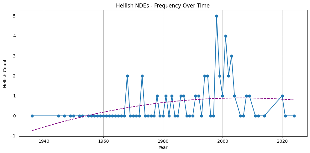
So this result is pretty weird and unexpected! Hellish NDEs do not appear to consistently increase or decrease, though there is a surprising cluster of hellish NDEs around the year 2000. Adding a quadratic model line indicates a gradual increase over time of hellish NDEs, though with diminishing returns.
I want to double check that the surprising peaks in the graph above are not due to there simply being more data for certain years, so I will now normalize the yearly counts (as I did with the previous analyses) and re-plot.
# normalize the data because some years just have more entries than others
normalization_vector = nde_experiences['year'].value_counts().sort_index().to_numpy()
print(normalization_vector)
[ 1  1  1  2  1  2  2  4  1  4  3  1  2  3  6  4  5  4  2  7  7  7  6  7
 11  6 15  8  9 11  9 12 12 16  6  9  7  9  7 10  9 10 19 12 14  5 11 14
 14 21 20 14 16 23 23 16 15  2  1  4  2  1  1  1  2  1  2]
# normalize the data because some years just have more entries than others
nde_experiences_time['ai_hellish_prop'] = nde_experiences_time['ai_hellish_count'] / normalization_vector
plt.figure(figsize=(10, 5))

# base scatterplot
plt.plot(nde_experiences_time['year'], nde_experiences_time['ai_hellish_prop'], marker='o')

# Fit quadratic polynomial
coeffs = np.polyfit(nde_experiences_time['year'], nde_experiences_time['ai_hellish_prop'], 2)
poly = np.poly1d(coeffs)

# Create smooth x values for plotting the curve
x_fit = np.linspace(nde_experiences_time['year'].min(), nde_experiences_time['year'].max(), 300)
y_fit = poly(x_fit)

# Plot quadratic fit
plt.plot(x_fit, y_fit, color='purple', linestyle='--',
         label='Quadratic fit')

plt.xlabel('Year')
plt.ylabel('Hellish Proportion')
plt.title('Hellish NDEs - Proportion Over Time')

plt.grid(True)
plt.tight_layout()

plt.show()
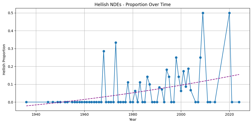
This final graph does indeed show that the peaks around the year 2000 had less to do with there being more hellish NDEs and more to do with there being more NDEs in general. Adding the quadratic model line indicates a steady increase in hellish NDEs over time, solidly contradicting my previous prediction!
Conclusion
It turns out that country and language are not very good predictors of NDE types. This is partly because there is a lack of variation in types of NDEs, with out-of-body experiences by far the most common type of NDE, consistently followed by extrasensory perception and feelings of unity or oneness. It is also because there is a paucity of data for countries other than Australia, Canada, France, and the US, as well as for languages other than English, French, and Spanish. Therefore to answer these questions better requires a more robust and inclusive dataset on NDEs.
That being said, I did discover that, contrary to my expectations, hellish NDEs have increased over time! This is a big surprising given the decline in religiosity over time, so further investigation of (a) what exactly comprisises a “hellish” NDE and (b) why these types of experiences are on the rise is certainly warranted.
Enjoy Reading This Article?
Here are some more articles you might like to read next: